| |
|
 |
CauseMap is an official Julia package.
To install, the user can simply type Pkg.add("CauseMap") from the Julia REPL.
CauseMap can then be imported with using CauseMap.
CauseMap is designed for rapid analysis. After setting a few tuning parameters (see Model Parameters), the user is ready to analyze and plot the results.
using CauseMap

# specify parameter ranges to test over
E_vals     = 2:10  # range to test of system dimensionality
tau_s_vals = 1:1 # range for lag length for manifold reconstruction
tau_p_vals = 0:15  # range to test for time lag of causal effect
#

# read in data
para, didi = load_example_data("ParaDidi")

# run analysis
makeoptimizationplots(para, didi,
                                        E_vals, tau_s_vals, tau_p_vals,
                                        "Para.", "Didi.";
                                        nreps=10, left_E=2, left_tau_p=0,   # optional
                                        right_E=7, right_tau_p=12, lagunit=.5, # optional
                                        unit="days", show_tau_s=false # optional
                                    )
This produces the plot below:
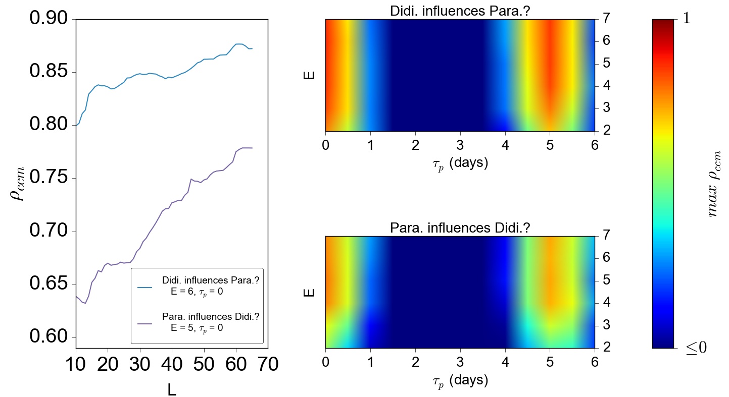
In the left panel, we see convergence for both causal directions. The interpretation of this result is that the causal relationship between P. aurelia and D. nasutum is bi-directional. That is, the number of predators influences the number of prey, and vice-versa.
The right panels show the dependence of the max ρccm on E (the dimensionality of the reconstructed system), and the supposed time lag of the causal effect (τp). Overall, the patterning of these heatmaps demonstrates that max ρccm has a reasonable dependence on causal parameters of interest. While the max ρccm is relatively insensitive to the assumed dimensionality, the best-performing τp values correspond to either immediate causal effects, or those delayed by five days.
Note that τp=5 corresponds to the principal frequency of the Paramecium aurelia and Didinium nasutum time series. This suggests that the peak at τp=5 is artifactual. Therefore, we are able to infer from these results that, as we would expect, predator and prey populations exert bidirectional effects in real-time.
For a look at the data behind this analysis, check out the interactive plots here.
Note that corresponding points can be simultaneously highlighted across plots using the select tool.
 CauseMap